Example Usage on ImageNet dataset

Example usages of EnsembleXAI package on the ImageNet dataset with usage of pretrained resnet50 model.

Imports of the necessary packages

import gc
import os
import json
import numpy as np
from PIL import Image
import urllib.request
import matplotlib.pyplot as plt
from matplotlib.colors import LinearSegmentedColormap
import torch
import torchvision.transforms.functional as F
from torchvision.transforms import Resize, CenterCrop
from torchvision.models import resnet50, ResNet50_Weights
from captum.attr import IntegratedGradients, Occlusion, NoiseTunnel, visualization as viz
from EnsembleXAI import Ensemble, Metrics

Setting paths to downloaded dataset

Below are some paths linking to data. Adjust them according to your directory setup. Data download process is available in Imagenet_data_prep.ipynb in the notebooks folder in repo (link)

input_dir = "\\".join(os.getcwd().split(sep="\\")[:-2] + ['input'])
#Correct path to masks and input is crucial, setup depends on users download path of the masks
masks_dir = input_dir + f'\\ImageNetS50\\train-semi-segmentation\\'
images_dir = "\\".join(os.getcwd().split(sep="\\")[:-1] + ['notebooks', 'images']) + "\\"

We can find natural names for each class id under this link.

with urllib.request.urlopen("https://s3.amazonaws.com/deep-learning-models/image-models/imagenet_class_index.json") as url:
    imagenet_classes_dict = json.load(url)

Helper functions to hasten the loading and the required image transformations.

def download_class_images(class_id, masks_path):
    full_path = os.path.join(masks_path, class_id)
    kaggle_path = f"/ILSVRC/Data/CLS-LOC/train/{class_id}/"
    for file_name in os.listdir(full_path):
        file_name_jpeg = file_name[:-3] + 'JPEG'
        !kaggle competitions download -f {kaggle_path}{file_name_jpeg} -p ./images/{class_id}/ -c imagenet-object-localization-challenge

def images_list(image_path, resize=True):
    _crop = CenterCrop(224).forward
    _resize = Resize([232,232]).forward
    images = []
    for image_name in os.listdir(image_path):
        image = Image.open(os.path.join(image_path, image_name))
        if resize:
            image = _crop(_resize(image))
        images.append(image)
    return images

def load_all(classid):
    all_img = images_list(os.path.join(images_dir, classid))[:3]
    all_img_org = images_list(os.path.join(images_dir, classid), resize=False)[:3]
    all_tens = [F.to_tensor(img) for img in all_img]
    all_msks = [(F.to_tensor(img)>0).float() for img in images_list(os.path.join(masks_dir, classid))[:3]]
    tens_img = torch.stack(all_tens)
    tens_msks = torch.stack(all_msks)
    return all_img, all_img_org, all_tens, all_msks, tens_img, tens_msks

Loading images and plotting the examples

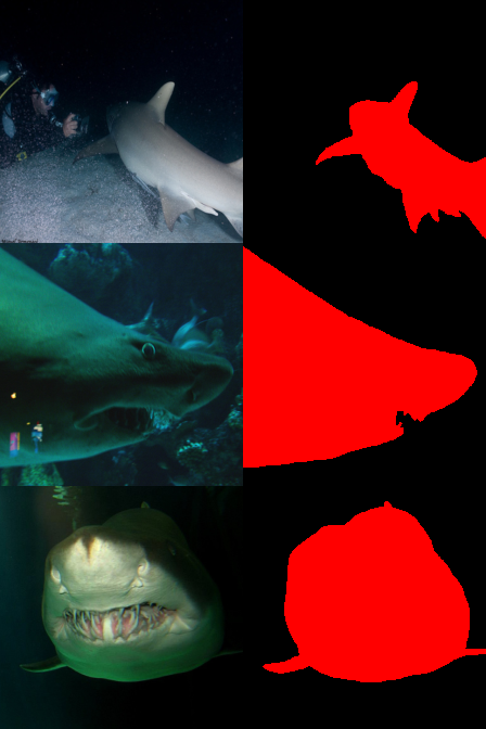
First setting up correct paths to masks and images is required. Masks are the ImageNetS50 masks found on (https://lusseg.github.io/, available under https://github.com/LUSSeg/ImageNet-S/releases/download/ImageNet-S/ImageNetS50-a0fe9d82231f9bc4787ee76e304dfa51.zip), consisting of 10 pixel-perfect masks for each of 50 classes sampled from the imagenet dataset. For sake of easier visualization, we consider 3 images from the “n01491361” class which is a tiger shark class.

#download single image from kaggle api, also available in func download_class_images()
os.mkdir(os.path.join('images'))
os.mkdir(os.path.join('images/n01491361'))
!kaggle competitions download -f "/ILSVRC/Data/CLS-LOC/train/n01491361/n01491361_1000.JPEG" -p ./images/n01491361/ -c imagenet-object-localization-challenge

id = "n01491361"
all_images, all_images_original, all_tensors, all_masks, tensor_images, tensor_masks = load_all("n01491361")

photos = []
for tensor, mask in zip(all_tensors, all_masks):
    photo = torch.cat([tensor, mask], dim=2)
    photos.append(photo)
display(F.to_pil_image(torch.cat(photos, dim=1)))

Model Loading

We use the resnet50 model pretrained on the imagenet dataset and generate predictions on our three images.

model = resnet50(weights=ResNet50_Weights.DEFAULT)
model.eval()
resnet_transform = ResNet50_Weights.DEFAULT.transforms()
pipeline = lambda images: torch.stack([resnet_transform(image) for image in images])
proper_data = pipeline(all_images_original)
outputs = model(proper_data)
_, preds = torch.max(outputs, 1)
probs2 = torch.nn.functional.softmax(outputs, dim=1)

Single Explanations

single_pred = preds[2].unsqueeze(dim=0)
single_data = proper_data[2].unsqueeze(dim=0)
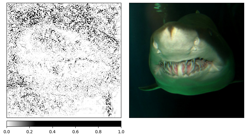
integrated_gradients = IntegratedGradients(model)
attributions_ig = integrated_gradients.attribute(single_data, target=single_pred, n_steps=200)
gc.collect()
transformed_img = resnet_transform(all_images_original[2])
default_cmap = LinearSegmentedColormap.from_list('custom blue',
                                                 [(0, '#ffffff'),
                                                  (0.25, '#000000'),
                                                  (1, '#000000')], N=256)
_1 = viz.visualize_image_attr_multiple(np.transpose(attributions_ig.squeeze().numpy(), (1,2,0)),
                                      np.transpose(tensor_images[2].squeeze().numpy(), (1,2,0)),
                                      ["heat_map", "original_image"],
                                      ["positive", "all"],
                                      cmap=default_cmap,
                                      show_colorbar=True,
                                      outlier_perc=1)

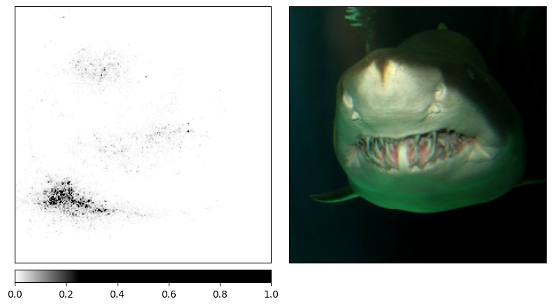
noise_tunnel = NoiseTunnel(integrated_gradients)
attributions_ig_nt = noise_tunnel.attribute(single_data, nt_samples=5, nt_type='smoothgrad_sq', target=single_pred)
gc.collect()
_2 = viz.visualize_image_attr_multiple(np.transpose(attributions_ig_nt.squeeze().numpy(), (1,2,0)),
                                      np.array(all_images[2]),
                                      ["heat_map", "original_image"],
                                      ["positive", "all"],
                                      cmap=default_cmap,
                                      show_colorbar=True)

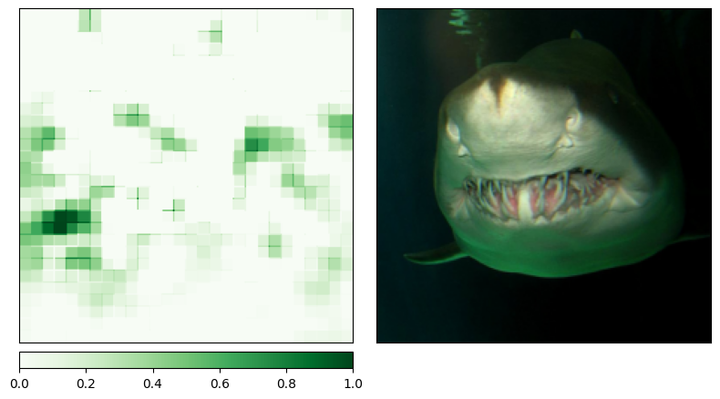
occlusion = Occlusion(model)
attributions_occ = occlusion.attribute(single_data,
                                       strides = (3, 8, 8),
                                       target=single_pred,
                                       sliding_window_shapes=(3, 15, 15),
                                       baselines=0)
_3 = viz.visualize_image_attr_multiple(np.transpose(attributions_occ.squeeze().cpu().detach().numpy(), (1,2,0)),
                                      np.array(all_images[2]),
                                      ["heat_map", "original_image"],
                                      ["positive", "all"],
                                      show_colorbar=True,
                                      outlier_perc=2,
                                      )

occlusion = Occlusion(model)

attributions_occ2 = occlusion.attribute(single_data,
                                       strides = (3, 20, 20),
                                       target=single_pred,
                                       sliding_window_shapes=(3, 25, 25),
                                       baselines=0)
_4 = viz.visualize_image_attr_multiple(np.transpose(attributions_occ2.squeeze().cpu().detach().numpy(), (1,2,0)),
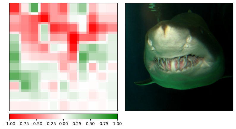
                                       np.array(all_images[2]),
                                       ["heat_map", "original_image"],
                                       ["all", "positive"],
                                       show_colorbar=True,
                                       outlier_perc=2,
                                       )

Explanations for all 3 images

Here we create example explanations for all 3 considered images.

occlusion = Occlusion(model)
attributions_occ_all_25 = occlusion.attribute(tensor_images,
                                        strides = (3, 20, 20),
                                        target = preds,
                                        sliding_window_shapes = (3, 25, 25),
                                        baselines=0)
attributions_occ_all_15 = occlusion.attribute(tensor_images,
                                           strides = (3, 8, 8),
                                           target = preds,
                                           sliding_window_shapes = (3, 15, 15),
                                           baselines=0)
attributions_ig_nt_all = torch.cat([noise_tunnel.attribute(tensor_images[i].unsqueeze(dim=0), nt_samples=5, nt_type='smoothgrad_sq', target=preds[i].unsqueeze(dim=0)) for i in range(tensor_images.shape[0])], dim=0)
gc.collect()

33356

Metrics for the created explanations

Calculation of consistency for the first image across both occlusion explanations.

Metrics.consistency(torch.stack([attributions_occ_all_15[0], attributions_occ_all_25[0]]))

0.03428497165441513

Calculation of decision impact ratio for occlusion25 explanations with threshold = 0.3. 0.33 result means that one third of the original images has change the decision after obscuring the critical area of explanation.

predict = lambda x: torch.nn.Softmax(dim=0)(model(x))
Metrics.decision_impact_ratio(tensor_images, predict, attributions_occ_all_25, 0.3, 0)

0.3333333432674408

Calculation of confidence impact ratio for occlusion25 explanations with threshold = 0.3. Negative value on “same_prediction” argument implies that on average the probability for the class predicted has increased after obscuring the critical area.

Metrics.confidence_impact_ratio(tensor_images, predict, attributions_occ_all_25, 0.3, 0, compare_to="same_prediction")

-0.004259963985532522

Calculation of confidence impact ratio for occlusion25 explanations with threshold = 0.3. Negative value on “new_prediction” argument implies that on average the maximal probability for the prediction has increased after obscuring the critical area.

Metrics.confidence_impact_ratio(tensor_images, predict, attributions_occ_all_25, 0.3, 0, compare_to="new_prediction")

-0.004277209285646677

Calculation of accordance recall for occlusion25. This metric calculates the area of explanation, mask intersection over the mask area. Therefore for the second image the explanation covers half of the mask area.

Metrics.accordance_recall(attributions_occ_all_25, tensor_masks)

tensor([0.3734, 0.5004, 0.2527])

Calculation of accordance precision for occlusion25. This metric calculates the area of explanation, mask intersection over the explanation area. Therefore for the second image the mask covers ~0.17 of the explanation area.

Metrics.accordance_precision(attributions_occ_all_25, tensor_masks)

tensor([0.0423, 0.1679, 0.1560])

Calculation of accordance F1 score for occlusion25. This is a average of harmonic averages of accordance precision and recall.

Metrics.F1_score(attributions_occ_all_25, tensor_masks)

0.1734609603881836

Calculation of average IOU for occlusion15.

Metrics.intersection_over_union(attributions_occ_all_15, tensor_masks)

0.0009072763496078551

def sample_xai(images):
    if images.shape[0] == 1:
        target = single_pred
    else:
        target = single_pred.repeat(images.shape[0])
    xai = occlusion.attribute(images,
                              strides = (3, 40, 40),
                              target=target,
                              sliding_window_shapes=(3,50, 50),
                              baselines=0)
    return xai
Metrics.stability(sample_xai, single_data.squeeze(dim=0), single_data.repeat(10,1,1,1))

0.0

Ensembles

Ensembling with the normEnsembleXAI functions across the 3 explanations.

all_stacked = torch.stack([attributions_ig_nt_all, attributions_occ_all_15, attributions_occ_all_25], dim=1)
aggreg_all1 = Ensemble.normEnsembleXAI(all_stacked, aggregating_func='avg')
aggreg_all2 = Ensemble.normEnsembleXAI(all_stacked, aggregating_func='min')
aggreg_all3 = Ensemble.normEnsembleXAI(all_stacked, aggregating_func='max')
explanations_all = torch.cat([all_stacked,aggreg_all3.unsqueeze(dim=1), aggreg_all2.unsqueeze(dim=1), aggreg_all1.unsqueeze(dim=1)], dim=1)

Consistency metric without and with the ensemblings.

[Metrics.consistency(all_stacked[i]) for i in range(all_stacked.shape[0])]

[0.018643660470843315, 0.03320877254009247, 0.04660186171531677]

[Metrics.consistency(explanations_all[i]) for i in range(explanations_all.shape[0])]

[0.015071503818035126, 0.022995971143245697, 0.032923243939876556]

Creating a model on the three photos. Of course it will not generalize at all, many more should be used for this to work properly, here presented as proof of concept.

res = Ensemble.supervisedXAI(explanations_all, tensor_masks[:,0], weights='auto', n_folds=2)

Metrics.intersection_over_union(res, tensor_masks[:,0])

0.32290786504745483

Metrics.accordance_recall(res, tensor_masks[:,0]), Metrics.accordance_precision(res, tensor_masks[:,0])

(tensor(0.6666), tensor(0.5122))

Metrics.confidence_impact_ratio(tensor_images, predict, res, 0.2, 0, compare_to="same_prediction")

0.22546647489070892

Plotting all explanations

plt.style.use('fast')
# helper function for the plotting
def plot_explanations(images, explanations, columns_names, classes_predicted, method = "heat_map"):
    cmaps=[default_cmap, None, None, None, None, None, None]
    nrow, ncol = len(images), explanations.shape[1]+1
    fig, ax = plt.subplots(nrows = nrow, ncols = ncol, figsize=(14, 3*explanations.shape[0]))
    for col, col_name in zip(ax[0], columns_names):
        col.title.set_text(col_name)
    for i, img in enumerate(images):
        ax[i,0].xaxis.set_ticks_position("none")
        ax[i,0].yaxis.set_ticks_position("none")
        ax[i,0].set_yticklabels([])
        ax[i,0].set_xticklabels([])
        ax[i,0].imshow(np.array(img), vmin=0, vmax=255)
        ax[i,0].set_ylabel(classes_predicted[i], size='large')
        for j, col in enumerate(ax[i,1:]):
            expl = explanations[i,j]
            sign = "positive"
            if expl.amin() < 0:
                sign = "all"
            _ = viz.visualize_image_attr(np.transpose(expl.squeeze().numpy(), (1,2,0)),
                                         original_image=np.array(img),
                                         method=method,
                                         sign=sign,
                                         plt_fig_axis=(fig, col),
                                         show_colorbar=True,
                                         outlier_perc=2,
                                         cmap=cmaps[j],
                                         use_pyplot=False
                                         )
    plt.show()

res2 = res.unsqueeze(dim=1).repeat(1,3,1,1)
predicted_names = [imagenet_classes_dict[str(i.item())][1] for i in preds]
col_names = ["Original", "Gradients", "Occlusion 25","Occlusion 15", "Max Aggregate", "Min Aggregate", "Avg", "KRR"]
plot_explanations(all_images, torch.cat([explanations_all,res.unsqueeze(dim=1)], dim=1), col_names, predicted_names, method="blended_heat_map")

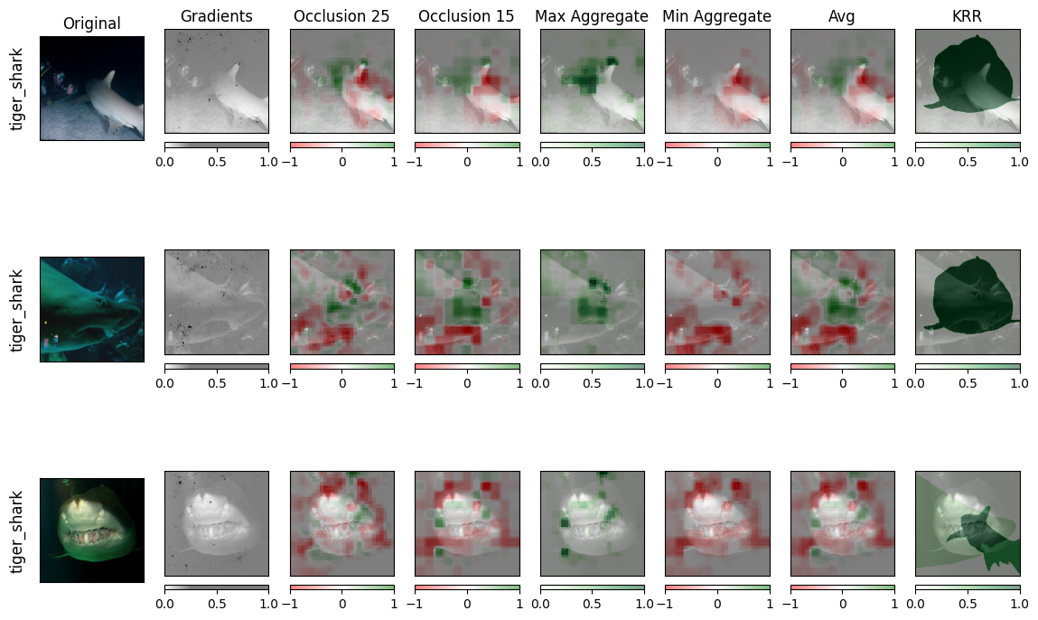
Here we can see the results as expected. In presence of non negative gradients explanation, max aggregate results in positive only values, while min aggregate results in nearly negative only explanation. Kernel Ridge Regression works as expected considering we only gave it 3 images with 2-folds cross validation.